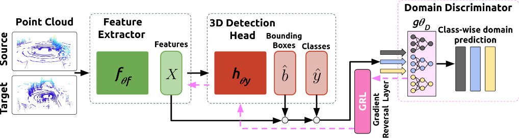
Detailed implementation of UADA3D The conditional module has the task of reducing the discrepancy between the condi- tional label distribution P (Ys|Xs) of the source and P (Yt|Xt) of the target. The label space Yi consists of class labels y ∈ RN ×K and 3D bounding boxes bi ∈ R7. The feature space X consists of point features F ∈ RN ×C (IA-SSD) or the 2D BEV pseudo- image I ∈ Rw×h×C (Centerpoint). The domain discriminator gθD in Centerpoint has 2D convolutional layers of 264, 256, 128, 1 while IA-SSD uses an MLP with dimensions 519, 512, 256, 128, 1. LeakyReLU is used for the activation functions with a sigmoid layer for the final domain prediction. A kernel size of 3 was chosen for Centerpoint, based on experiments shown in B.4. Note, that we do class-wise domain prediction, thus we have K discriminators corresponding to the number of classes (in our case K = 3, but it can be easily modified).

Detailed implementation of UADA3D_Lm The primary role UADA3D_Lm with the marginal feature discriminator is to minimize the discrepancy between the marginal feature distributions of the source, denoted as P(X_s), and the target, represented by P(X_t). Here, X_s and X_t symbolize the features extracted by the detection backbone from the two distinct domains. This approach ensures the extraction of domain invariant features. The loss function of UADA3D_Lm marginal alignment module is defined through Binary Cross Entropy. The output of the point-based detection backbone in IA-SSD is given by N point features with feature dimension C and corresponding encodings. Point-wise discriminators can be utilized to identify the distribution these points are drawn from. The input to the proposed marginal discriminator \( g_{\theta_D} \) is given by point-wise center features obtained through set abstraction and downsampling layers. The discriminator is made up of 5 fully connected layers (512,256,128,64,32,1 ) that reduce the feature dimension from C to 1 . LeakyReLU is used in the activation layers and a final sigmoid layer is used for domain prediction. The backbone in Centerpoint uses sparse convolutions to extract voxel-based features that are flattened into 2D BEV-features. Therefore, the input to the view-based marginal discriminator is given by a pseudo image of feature dimension C with spatial dimensions \(w\) and \(h\) that define the 2D BEV-grid. Since 2D convolutions are more computationally demanding over the MLP on the heavily downsampled point cloud in IA-SSD">IA-SSDD_Lm, the 2D marginal discriminator uses a \(3\)-layered CNN that reduces the feature dimension from C to 1 (256,256,128,1), using a kernel size of 3 and a stride of 1. Same as in the point-wise case, the loss function of UADA3D_Lm is defined through Cross Entropy.

In ablation studies we tested two different strategies for GRL-coefficient \( \lambda \) on UADA3D and UADA3DLm. Firstly, a stationary \( \lambda=0.1 \) was tested following the setting used for most adversarial UDA strategies in 2D object detection. Secondly, we follow other approaches where \( \lambda \) was increased over the training according to: \begin{equation} \label{eq:params-grl} \lambda = \alpha (\frac{2}{1 + exp(-\gamma p)} - 1) \end{equation} where \( \alpha \in [0,1] \) is a scaling factor that determines the final \( \lambda \), \( \gamma \) =10 and p is the training progress from start \(0\) to finish \(1\). \( \alpha \)values of 1, 0.5, 0.2, 0.1 were tested. The \( \lambda \) parameter for different values of \( \alpha \) throughout training process is illustrated in graph below. Numerical results regarding the influence of \( \lambda \) on the model performance are available in Section 5.1 Ablation Studies.

Random Object Scaling (ROS) applies random scaling factors to ground truth bounding boxes and their corresponding points. Each object point in ego-vehicle frame \( (p_i^x,p_i^y,p_i^z)_{\mathrm{ego}} \) is transformed to local object coordinates \begin{equation} \begin{array}{cc} (p_i^l,p_i^w,p_i^h)_{\mathrm{object}} = ((p_i^x,p_i^y,p_i^z)_{\mathrm{ego}} - \\ ~~~~~~~~~~~~~~(c_x,c_y,c_z)_{\mathrm{object}}) \times R_{\mathrm{object}} \end{array} \end{equation} \noindent where \( (c_x,c_y,c_z)_{\mathrm{object}} \) is object center coordinates and \(R_{\mathrm{object}}\) is the rotation matrix between the ego-coordinates and object-coordinates. Each object point is then scaled by a random scaling factor \(r\) drawn from a uniform random distribution: The length \(l\), width \(w\), and height \(h\) of each bounding box are also scaled accordingly with \(r\). \begin{equation} \begin{array}{cc} (p_i^l,p_i^w,p_i^h)_{\mathrm{object},\mathrm{scaled}} = r \cdot (p_i^l,p_i^w,p_i^h)_{\mathrm{object}} \; \\ r \in U(r_{\mathrm{min}},r_{\mathrm{max}}). \end{array} \end{equation}

Afterwards, each object is transformed back into the ego-vehicle frame. The length \(l\), width \(w\), and height \(h\) of each bounding box are also scaled accordingly with \(r\). Following previous works experiments are performed by including object scaling in the source-data to account for different vehicle sizes. As examined in Section 4.1 there is a large difference between the vehicle sizes in LiDAR-CS, corresponding to large vehicle sizes typically found in the USA, and the smaller vehicles in Europe encountered by the robot, which encounters the smaller vehicles in Europe. Specifically, ROS from ST3D~\cite{yang2021st3d} is utilized where the objects and corresponding bounding boxes are scaled according to uniform noise in a chosen scaling interval. While previous UDA methods on LiDAR-based 3D object detection often apply domain adaptation only to a single object category, we consider it a multiclass problem. Therefore, ROS is used for all three classes (Vehicle, Pedestrian, and Cyclist) with different scaling intervals, shown in~\cref{tab:ros_scale}. The results of different scaling intervals are shown in table below. We can see that the best setting is \(\Delta_{x,y,z} \in \{0.80,1.20\}\) for vehicles and \(\Delta_{x,y,z} \in \{0.9,1.1\}\) for pedestrians and cyclists, thus, we chose this for all of our experiments.

Motivated by other works, we try to use a few labels from target data to see if that can further improve our results. In Table below, we present results across three scenarios. Interestingly, we observed some improvements, particularly in adaptation towards robot data, and slight enhancements in other datasets, although not as pronounced. This could be attributed to robot data being smaller than nuScenes. Notably, we observed particularly high improvements in the Pedestrian and Cyclist classes. Moreover, we found that adding W → N led to higher improvements than CS64 → N. Remarkably, we achieved these results using only 20 labeled target examples for this few-shot approach.

The mobile robot used to capture robot data is a wheeled last-mile delivery robot developed at TU Hamburg (see Figure 10). It is equipped with a Intel Core i7-7600U 2x2.80 GHz CPU and a NVIDIA Volta GPU with 64 Tensor cores. Its sensors consist of two forward and backward facing Stereolabs ZED2 stereo cameras, four Intel RealSense D435 stereo cameras in the downward direction as well as a 16-channel Velodyne Puck (VLP-16) LiDAR. Since this work concerns LiDAR-based detection, only the LiDAR sensor is used for detection in this work.

The training data was collected at the campuses and the neighborhoods During training and testing the data was randomly sampled from these two locations. Our dataset includes sequences from both outdoor (university sidewalks, small university roads, or parking lots) and indoor (the university building and a warehouse) scenarios. Most of the objects classes in these areas are pedestrians and cyclists. There are also numerous vehicles, mostly parked on the side of the road or driving across the university campus. Since the data was collected in scenarios similar to the intended use cases for such robots it can be seen as an accurate representation of the data that would be encountered in real-world operation. The data was labeled using the open-source annotation software SUSTechPoints. In our train/test split, we used a similar number of scans as on the KITTI data. We used 7000 scans for training and 3500 for testing. Together with this paper, we are planning to release the robot data we used in our scenarios. The complete dataset is a part of another project and will be published soon. In addition to the LiDAR data and class labels (used in this project), the full dataset will also include data from an RGBD camera, ground-facing stereo camera, an Inertial Measurement Unit (IMU), wheel odometry, and RTK GNSS. This diverse collection of sensors will offer a comprehensive perspective on the robot’s perception of its environment, providing valuable insights into the subtle aspects of robotic sensing capabilities.

The loss of our network consists of 2 components: detection loss and discriminator loss. While we optimize the discriminators with L_C, we backpropagate this loss through the gradient reversal layer to the rest of the network. Thus, while the discriminator's objective is to minimize \(\mathcal{L}_C\), the feature extractor and detection head benefit from maximizing \(\mathcal{L}_C\). In other words, the network aims to create features that are domain-invariant and useful for the object detection task. We can observe these losses in figure below. Initially, we can see that the discriminator is capable of distinguishing between the domains as the loss decreases and approaches 0. However, after approximately 30\% of the training, the network begins to produce more invariant features. By about 40\% of the training, the network has learned to generate invariant features, leading to a rapid increase in conditional discriminator loss. These features are still beneficial for detection, resulting in a decrease in detection loss and a rapid overall loss reduction until the conditional discriminator loss plateaus again.

Our method, UADA3D, demonstrated the ability to accurately train the model to recognize objects, irrespective of their proximity and domain. This enhanced detection capability is effective across all three classes: vehicles, pedestrians, and cyclists. Our approach significantly improves the model's ability to identify distant, close-by as well as heavily occluded objects. In the next figures, red bounding boxes indicate predictions, while green bounding boxes represent ground truth. We added blue squares to highlight zoomed-in regions, and yellow dotted squares to highlight hard-to-detect far-away objects. As illustrated in figures below, most of the models in comparison tend to miss far-away or partially occluded objects, without producing many false positives. Additionally, they also tend to miss smaller non-vehicle objects. UADA3D on the other hand substantially enhances the model's robustness in these challenging scenarios, ensuring that such objects are not overlooked. Our method detects not only close and far away vehicles (see figures) but also hard-to-see cyclists and pedestrians (zoomed-in regions in figures below, as well as highlighted with the yellow box containing one instance). Moreover, in the figures with results on robot data, which presents results on robot data, we show UADA3D's comprehensive adaptation capabilities, where we successfully identify every object in the scene, even though the domain gap is substantially large (self-driving car domain to mobile robot). This highlights the effectiveness of our approach in diverse and demanding real-world applications.